Hadronic pp jet model
In this section we show the hadronic pp implemented for the Jet model. The pp implementation is based on the work presented in [Kelner2006].
Secondaries \(e^{\pm}\), are evolved to the equilibrium following the approach in [Inoue96]. To speed up the process only synchroton cooling is taken into account. In the next release also the option to switch on IC cooling contribution will be added.
A validation of the integral solution for the \(e^{\pm}\) equilibrium used for the pp jet against the Fokker-Plank equation solution, implemented in the JetTimeEvol class, is presented in Validation of the pp equilibrium against the Fokker-Plank equation solution
We remind the approximation of the only synchrotron cooling is used only for this specific class, and for this first release, and that the JetTimeEvol class offers full cooling access (synchrotron, IC, and adiabatic expansion). See temporal evolution for more details.
from jetset.jet_model import Jet
from jetset.jetkernel import jetkernel
from astropy import constants as const
from jetset.jet_emitters_factory import EmittersFactory
import matplotlib.pyplot as plt
import numpy as np
def get_component(j_name,nu_name):
    j_nu_ptr=getattr(j._blob,j_name)
    nu_ptr=getattr(j._blob,nu_name)
    xg=np.zeros(j._blob.nu_grid_size)
    yg=np.zeros(j._blob.nu_grid_size)
    for i in range(j._blob.nu_grid_size):
        xg[i]=jetkernel.get_spectral_array(nu_ptr,j._blob,i)
        yg[i]=jetkernel.get_spectral_array(j_nu_ptr,j._blob,i)

    m=yg>0

    xg=xg[m]
    yg=yg[m]
    yg=yg*xg
    yg=yg*jetkernel.erg_to_TeV

    xg=xg*jetkernel.HPLANCK_TeV

    return xg,yg
import jetset
print('tested on jetset',jetset.__version__)
tested on jetset 1.2.0
To get an hadronic jet with pp interaction, we set the
emitters_type='protons'
j=Jet(emitters_distribution='plc',verbose=False,emitters_type='protons')
j.parameters.R.val=1E16
j.parameters.N.val=1000
j.parameters.B.val=1
j.parameters.z_cosm.val=0.001
j.parameters.beam_obj.val=20
j.eval()
j.show_model()
--------------------------------------------------------------------------------
jet model description
--------------------------------------------------------------------------------
name: jet_hadronic_pp

protons distribution:
 type: plc
 gamma energy grid size:  201
 gmin grid : 2.000000e+00
 gmax grid : 1.000000e+06
 normalization  True
 log-values  False

radiative fields:
 seed photons grid size:  100
 IC emission grid size:  100
 source emissivity lower bound :  1.000000e-120
 spectral components:
   name:Sum, state: on
   name:Sync, state: self-abs
   name:SSC, state: on
   name:PP_gamma, state: on
   name:PP_neutrino_tot, state: on
   name:PP_neutrino_mu, state: on
   name:PP_neutrino_e, state: on
   name:Bremss_ep, state: on
external fields transformation method: blob

SED info:
 nu grid size jetkernel: 1000
 nu size: 500
 nu mix (Hz): 1.000000e+06
 nu max (Hz): 1.000000e+30

flux plot lower bound   :  1.000000e-30

--------------------------------------------------------------------------------
| model name | name | par type | units | val | phys. bound. min | phys. bound. max | log | frozen |
|---|---|---|---|---|---|---|---|---|
| jet_hadronic_pp | R | region_size | cm | 1.000000e+16 | 1.000000e+03 | 1.000000e+30 | False | False |
| jet_hadronic_pp | R_H | region_position | cm | 1.000000e+17 | 0.000000e+00 | -- | False | True |
| jet_hadronic_pp | B | magnetic_field | gauss | 1.000000e+00 | 0.000000e+00 | -- | False | False |
| jet_hadronic_pp | beam_obj | beaming | lorentz-factor* | 2.000000e+01 | 1.000000e-04 | -- | False | False |
| jet_hadronic_pp | z_cosm | redshift | 1.000000e-03 | 0.000000e+00 | -- | False | False | |
| jet_hadronic_pp | gmin | low-energy-cut-off | lorentz-factor* | 2.000000e+00 | 1.000000e+00 | 1.000000e+09 | False | False |
| jet_hadronic_pp | gmax | high-energy-cut-off | lorentz-factor* | 1.000000e+06 | 1.000000e+00 | 1.000000e+15 | False | False |
| jet_hadronic_pp | N | emitters_density | 1 / cm3 | 1.000000e+03 | 0.000000e+00 | -- | False | False |
| jet_hadronic_pp | NH_pp | target_density | 1 / cm3 | 1.000000e+00 | 0.000000e+00 | -- | False | False |
| jet_hadronic_pp | gamma_cut | turn-over-energy | lorentz-factor* | 1.000000e+04 | 1.000000e+00 | 1.000000e+09 | False | False |
| jet_hadronic_pp | p | LE_spectral_slope | 2.000000e+00 | -1.000000e+01 | 1.000000e+01 | False | False |
--------------------------------------------------------------------------------
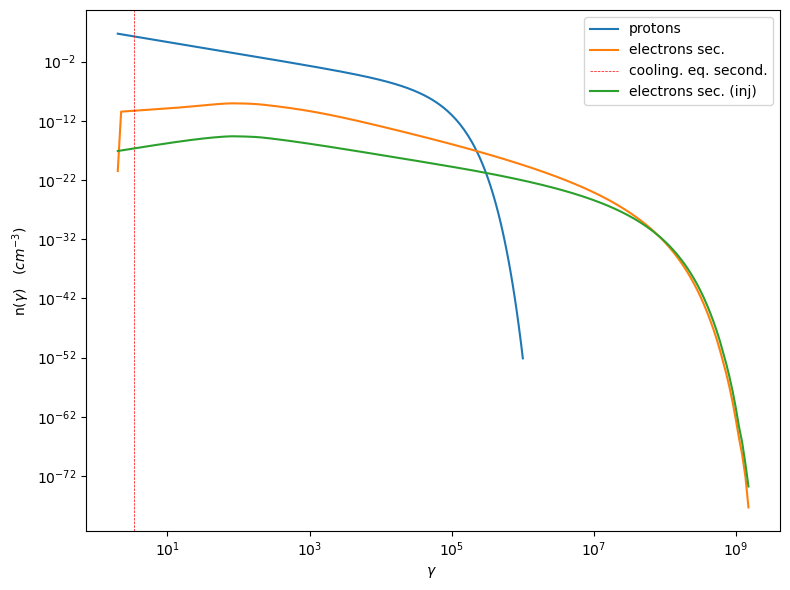
gmin=1.0/jetkernel.MPC2_TeV
m=j.emitters_distribution.gamma_p>=gmin
print('U(p) (erg/cm3) =',j.emitters_distribution.eval_U(gmin=gmin))
U(p) (erg/cm3) = 5.257679637585933
%matplotlib inline
p=j.emitters_distribution.plot()
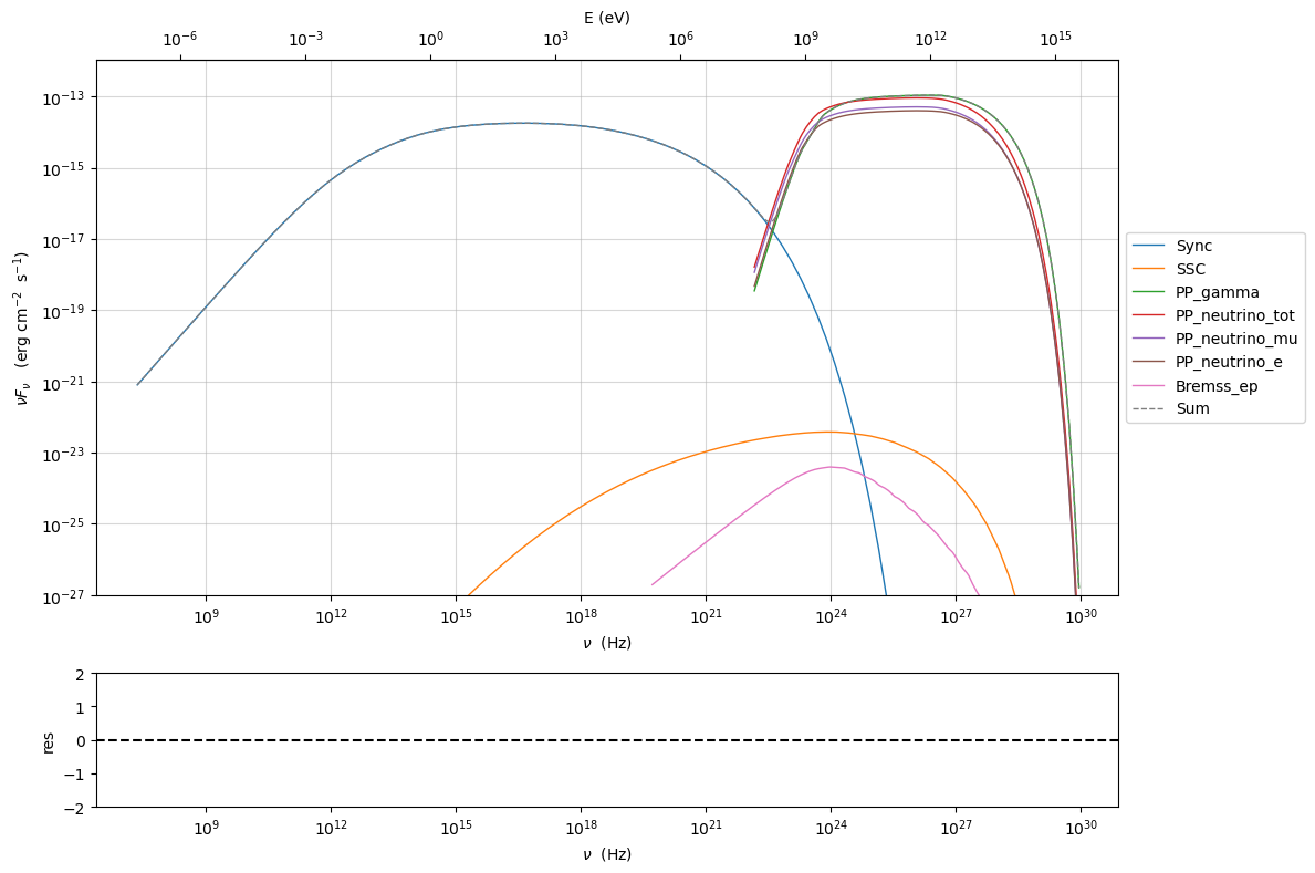
%matplotlib inline
p=j.plot_model()
p.setlim(y_min=1E-27)
Jet pp Consistency with Kelner 2006
j=Jet(emitters_distribution='plc',verbose=False,emitters_type='protons')
j.parameters.z_cosm.val=z=0.001
j.parameters.beam_obj.val=10
j.parameters.gamma_cut.val=1000/(jetkernel.MPC2_TeV)
j.parameters.NH_pp.val=1
j.parameters.N.val=1
j.parameters.p.val=2.0
j.parameters.B.val=1.0
j.parameters.R.val=1E18
j.parameters.gmin.val=1
j.parameters.gmax.val=1E8
j.set_emiss_lim(1E-60)
j.set_IC_nu_size(100)
j.gamma_grid_size=200
j.nu_max=1E31
gamma_sec_evovled=np.copy(j.emitters_distribution.gamma_e)
n_gamma_sec_evovled=np.copy(j.emitters_distribution.n_gamma_e)
gamma_sec_inj=np.copy(j.emitters_distribution.gamma_e_second_inj)
n_gamma_sec_inj=np.copy(j.emitters_distribution.n_gamma_e_second_inj)
gmin=1.0/jetkernel.MPC2_TeV
j.set_N_from_U_emitters(1.0, gmin=gmin)
j.eval()
j.show_model()
--------------------------------------------------------------------------------
jet model description
--------------------------------------------------------------------------------
name: jet_hadronic_pp

protons distribution:
 type: plc
 gamma energy grid size:  201
 gmin grid : 1.000000e+00
 gmax grid : 1.000000e+08
 normalization  True
 log-values  False

radiative fields:
 seed photons grid size:  100
 IC emission grid size:  100
 source emissivity lower bound :  1.000000e-60
 spectral components:
   name:Sum, state: on
   name:Sync, state: self-abs
   name:SSC, state: on
   name:PP_gamma, state: on
   name:PP_neutrino_tot, state: on
   name:PP_neutrino_mu, state: on
   name:PP_neutrino_e, state: on
   name:Bremss_ep, state: on
external fields transformation method: blob

SED info:
 nu grid size jetkernel: 1000
 nu size: 500
 nu mix (Hz): 1.000000e+06
 nu max (Hz): 1.000000e+31

flux plot lower bound   :  1.000000e-30

--------------------------------------------------------------------------------
| model name | name | par type | units | val | phys. bound. min | phys. bound. max | log | frozen |
|---|---|---|---|---|---|---|---|---|
| jet_hadronic_pp | R | region_size | cm | 1.000000e+18 | 1.000000e+03 | 1.000000e+30 | False | False |
| jet_hadronic_pp | R_H | region_position | cm | 1.000000e+17 | 0.000000e+00 | -- | False | True |
| jet_hadronic_pp | B | magnetic_field | gauss | 1.000000e+00 | 0.000000e+00 | -- | False | False |
| jet_hadronic_pp | beam_obj | beaming | lorentz-factor* | 1.000000e+01 | 1.000000e-04 | -- | False | False |
| jet_hadronic_pp | z_cosm | redshift | 1.000000e-03 | 0.000000e+00 | -- | False | False | |
| jet_hadronic_pp | gmin | low-energy-cut-off | lorentz-factor* | 1.000000e+00 | 1.000000e+00 | 1.000000e+09 | False | False |
| jet_hadronic_pp | gmax | high-energy-cut-off | lorentz-factor* | 1.000000e+08 | 1.000000e+00 | 1.000000e+15 | False | False |
| jet_hadronic_pp | N | emitters_density | 1 / cm3 | 1.058009e+02 | 0.000000e+00 | -- | False | False |
| jet_hadronic_pp | NH_pp | target_density | 1 / cm3 | 1.000000e+00 | 0.000000e+00 | -- | False | False |
| jet_hadronic_pp | gamma_cut | turn-over-energy | lorentz-factor* | 1.065789e+06 | 1.000000e+00 | 1.000000e+09 | False | False |
| jet_hadronic_pp | p | LE_spectral_slope | 2.000000e+00 | -1.000000e+01 | 1.000000e+01 | False | False |
--------------------------------------------------------------------------------
m=j.emitters_distribution.gamma_p>=gmin
print('U(p) (erg/cm3) =',j.emitters_distribution.eval_U(gmin=gmin))
U(p) (erg/cm3) = 1.0
%matplotlib inline
p=j.emitters_distribution.plot()
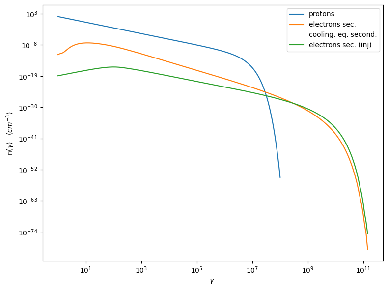
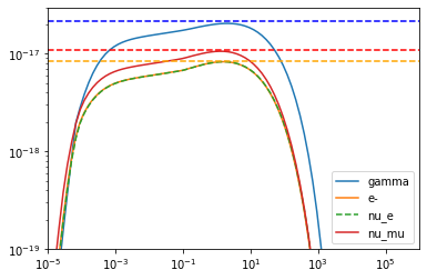
#Fig 12 Kelner 2006
%matplotlib inline


#j_nu_pp rate
xg,yg= get_component('j_pp_gamma','nu_pp_gamma')
x_nu_e,y_nu_e= get_component('j_pp_neutrino_e','nu_pp_neutrino_e')
x_nu_mu,y_nu_mu= get_component('j_pp_neutrino_mu','nu_pp_neutrino_mu')
x_nu_tot,y_nu_tot= get_component('j_pp_neutrino_tot','nu_pp_neutrino_tot')
x_nu_mu_2=x_nu_mu
y_nu_2=(y_nu_tot-y_nu_mu)*np.pi*4
x_nu_mu_1=x_nu_mu
y_nu_mu_1=(y_nu_mu-y_nu_2)*np.pi*4

yg=yg*np.pi*4
y_nu_mu=y_nu_mu*np.pi*4
y_nu_e=y_nu_e*np.pi*4
#e-  rate
x_inj=np.copy(j.emitters_distribution.gamma_e_second_inj)
y_inj=np.copy(j.emitters_distribution.n_gamma_e_second_inj)
y_e=y_inj*x_inj*x_inj*jetkernel.MEC2_TeV
x_e=x_inj*0.5E6/1E12

plt.loglog(xg,yg,label='gamma')
plt.loglog(x_e,y_e,label='e-')
plt.loglog(x_nu_e,y_nu_e,'--',label='nu_e')
plt.loglog(x_nu_mu,y_nu_mu,label='nu_mu')

#plt.loglog(x_nu_mu_1,y_nu_mu_1,label='nu_mu_1')

plt.ylim(1E-19,3E-17)#
plt.xlim(1E-5,1E6)

plt.legend()
plt.axhline(2.15E-17,ls='--',c='b')
plt.axhline(8.5E-18,ls='--',c='orange')
plt.axhline(1.1E-17,ls='--',c='r')
<matplotlib.lines.Line2D at 0x7fbc161dbca0>
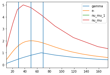
#Fig 14 left panel
%matplotlib inline
y1=yg/(xg*xg)
plt.plot(xg*1E6,y1/y1.max(),label='gamma')

y1=y_e/(x_e*x_e)
m=y_e>0
plt.plot(x_e[m]*1E6,2*y1[m]/y1[m].max(),label='e-')

#y1=y_nu_tot/(x_nu_tot*x_nu_tot)
#m=y1>0
#plt.plot(x_nu_tot[m]*1E6,3*y1[m]/y1[m].max(),label='nu_tot')
y1=y_nu_mu_1/(x_nu_mu_1*x_nu_mu_1)
m=y1>0
plt.plot(x_nu_mu_1[m]*1E6,4*y1[m]/y1[m].max(),label='nu_mu_1')

y1=y_nu_mu/(x_nu_mu*x_nu_mu)
m=y1>0
plt.plot(x_nu_mu[m]*1E6,5*y1[m]/y1[m].max(),label='nu_mu')

#plt.xlim(1E-5,2E2)
plt.axvline(70)
plt.axvline(50)
plt.axvline(30)
plt.legend()
plt.xlim(10,175)
(10.0, 175.0)