Validation of the pp equilibrium against the Fokker-Plank equation solution

In this tutorial we validate the integral solution for the \(e^{\pm}\) equilibrium, used for the pp jet against the Fokker-Plank equation solution implemented in the JetTimeEvol class (see the Hadronic pp jet model, for more details on the pp hadronic jet model)

Jet pp

from jetset.jet_model import Jet
from jetset.jetkernel import jetkernel
from astropy import constants as const
from jetset.jet_emitters_factory import EmittersFactory
from jetset.jet_emitters import InjEmittersArrayDistribution
import numpy as np
import matplotlib.pyplot as plt

def get_component(j_name,nu_name):
    j_nu_ptr=getattr(j._blob,j_name)
    nu_ptr=getattr(j._blob,nu_name)
    xg=np.zeros(j._blob.nu_grid_size)
    yg=np.zeros(j._blob.nu_grid_size)
    for i in range(j._blob.nu_grid_size):
        xg[i]=jetkernel.get_spectral_array(nu_ptr,j._blob,i)
        yg[i]=jetkernel.get_spectral_array(j_nu_ptr,j._blob,i)

    m=yg>0

    xg=xg[m]
    yg=yg[m]
    yg=yg*xg
    yg=yg*jetkernel.erg_to_TeV

    xg=xg*jetkernel.HPLANCK_TeV

    return xg,yg

import jetset
print('tested on jetset',jetset.__version__)

tested on jetset 1.2.0

j=Jet(emitters_distribution='plc',verbose=False,emitters_type='protons')

j.parameters.z_cosm.val=z=0.001
j.parameters.beam_obj.val=1
j.parameters.gamma_cut.val=1000/(jetkernel.MPC2_TeV)
j.parameters.NH_pp.val=1
j.parameters.N.val=1
j.parameters.p.val=2.0
j.parameters.B.val=.5
j.parameters.R.val=1E18
j.parameters.gmin.val=1
j.parameters.gmax.val=1E4
j.set_emiss_lim(1E-60)
j.set_IC_nu_size(100)
j.gamma_grid_size=200
j.eval()

gmin=1.0/jetkernel.MPC2_TeV
j.set_N_from_U_emitters(1.0, gmin=gmin)
j.eval()

#j.show_model()

m=j.emitters_distribution.gamma_p>gmin
print('U N(p) p>1 TeV=%e erg/cm-3'%(jetkernel.MPC2*np.trapz(j.emitters_distribution.n_gamma_p[m]*j.emitters_distribution.gamma_p[m],j.emitters_distribution.gamma_p[m])))

U N(p) p>1 TeV=9.999992e-01 erg/cm-3

j.energetic_report(verbose=False)

%matplotlib inline
j.emitters_distribution.plot()

<jetset.plot_sedfit.PlotPdistr at 0x7fc5c3373fd0>

j.save_model('hadronic.pkl')

from jetset.jet_model import Jet
j=Jet.load_model('hadronic.pkl')

Table length=11

model name	name	par type	units	val	phys. bound. min	phys. bound. max	log	frozen
jet_hadronic_pp	gmin	low-energy-cut-off	lorentz-factor*	1.000000e+00	1.000000e+00	1.000000e+09	False	False
jet_hadronic_pp	gmax	high-energy-cut-off	lorentz-factor*	1.000000e+04	1.000000e+00	1.000000e+15	False	False
jet_hadronic_pp	N	emitters_density	1 / cm3	3.022554e+02	0.000000e+00	--	False	False
jet_hadronic_pp	NH_pp	target_density	1 / cm3	1.000000e+00	0.000000e+00	--	False	False
jet_hadronic_pp	gamma_cut	turn-over-energy	lorentz-factor*	1.065789e+06	1.000000e+00	1.000000e+09	False	False
jet_hadronic_pp	p	LE_spectral_slope		2.000000e+00	-1.000000e+01	1.000000e+01	False	False
jet_hadronic_pp	R	region_size	cm	1.000000e+18	1.000000e+03	1.000000e+30	False	False
jet_hadronic_pp	R_H	region_position	cm	1.000000e+17	0.000000e+00	--	False	True
jet_hadronic_pp	B	magnetic_field	gauss	5.000000e-01	0.000000e+00	--	False	False
jet_hadronic_pp	beam_obj	beaming	lorentz-factor*	1.000000e+00	1.000000e-04	--	False	False
jet_hadronic_pp	z_cosm	redshift		1.000000e-03	0.000000e+00	--	False	False

setting up the JetTimeEvol model

gamma_sec_evovled=np.copy(j.emitters_distribution.gamma_e)
n_gamma_sec_evovled=np.copy(j.emitters_distribution.n_gamma_e)
gamma_sec_inj=np.copy(j.emitters_distribution.gamma_e_second_inj)
n_gamma_sec_inj=np.copy(j.emitters_distribution.n_gamma_e_second_inj)

from jetset.jet_emitters_factory import EmittersFactory
from jetset.jet_emitters import InjEmittersArrayDistribution
q_inj=InjEmittersArrayDistribution(name='array_distr',emitters_type='electrons',gamma_array=gamma_sec_inj,n_gamma_array=n_gamma_sec_inj,normalize=False)

q_inj.parameters

Table length=3

name	par type	units	val	phys. bound. min	phys. bound. max	log	frozen
gmin	low-energy-cut-off	lorentz-factor*	1.000000e+00	1.000000e+00	1.000000e+09	False	False
gmax	high-energy-cut-off	lorentz-factor*	1.836150e+07	1.000000e+00	1.000000e+15	False	False
Q	emitters_density	1 / (cm3 s)	1.000000e+00	0.000000e+00	--	False	False

None

%matplotlib inline
p=q_inj.plot()
p.ax.plot(gamma_sec_inj, n_gamma_sec_inj,'.',ms=1.5)

[<matplotlib.lines.Line2D at 0x7fc5c471fd90>]

from jetset.jet_timedep import JetTimeEvol
from jetset.jet_model import Jet

temp_ev=JetTimeEvol(jet_rad=j,Q_inj=q_inj,only_radiation=True,inplace=True)

/Users/orion/anaconda3/envs/jetset/lib/python3.8/site-packages/jetset/model_manager.py:147: UserWarning: no cosmology defined, using default FlatLambdaCDM(name="Planck13", H0=67.8 km / (Mpc s), Om0=0.307, Tcmb0=2.725 K, Neff=3.05, m_nu=[0.   0.   0.06] eV, Ob0=0.0483)
  warnings.warn('no cosmology defined, using default %s'%self.cosmo)

temp_ev.Q_inj.parameters.Q.val

1

we use the acc region with escape time equal to radiative region

duration=5E9
duration_acc=0
T_SIZE=np.int(2E6)

temp_ev.parameters.duration.val=duration

temp_ev.parameters.TStart_Inj.val=0
temp_ev.parameters.TStop_Inj.val=duration
temp_ev.parameters.T_esc_rad.val= 1


temp_ev.parameters.Esc_Index_rad.val=0
temp_ev.parameters.t_size.val=T_SIZE
temp_ev.parameters.num_samples.val=500
temp_ev.IC_cooling='off'
temp_ev.parameters.L_inj.val=0

temp_ev.parameters.gmin_grid.val=1.1
temp_ev.parameters.gmax_grid.val=5E7
temp_ev.parameters.gamma_grid_size.val=400

temp_ev.init_TempEv()
temp_ev.region_expansion='off'
temp_ev.show_model()

--------------------------------------------------------------------------------
JetTimeEvol model description
--------------------------------------------------------------------------------

physical setup:

--------------------------------------------------------------------------------

Table length=12

name	par type	val	units	val*	units*	log
delta t	time	2.500000e+03	s	7.494811449999999e-05	R/c	False
log. sampling	time	0.000000e+00		None		False
R/c	time	3.335641e+07	s	1.0	R/c	False
IC cooling		off		None		False
Sync cooling		on		None		False
Adiab. cooling		on		None		False
Reg. expansion		off		None		False
Tesc rad	time	3.335641e+07	s	1.0	R/c	False
R_rad rad start	region_position	1.000000e+18	cm	None		False
R_H rad start	region_position	1.000000e+17	cm	None		False
T min. synch. cooling		6.190400e+01	s	None		False
L inj (electrons)	injected lum.	7.490407e+38	erg/s	None		False

model parameters:

--------------------------------------------------------------------------------

Table length=17

model name	name	par type	units	val	phys. bound. min	phys. bound. max	log	frozen
jet_time_ev	duration	time_grid	s	5.000000e+09	0.000000e+00	--	False	True
jet_time_ev	gmin_grid	gamma_grid		1.100000e+00	0.000000e+00	--	False	True
jet_time_ev	gmax_grid	gamma_grid		5.000000e+07	0.000000e+00	--	False	True
jet_time_ev	gamma_grid_size	gamma_grid		4.000000e+02	0.000000e+00	--	False	True
jet_time_ev	TStart_Inj	time_grid	s	0.000000e+00	0.000000e+00	--	False	True
jet_time_ev	TStop_Inj	time_grid	s	5.000000e+09	0.000000e+00	--	False	True
jet_time_ev	T_esc_rad	escape_time	(R/c)*	1.000000e+00	--	--	False	True
jet_time_ev	Esc_Index_rad	fp_coeff_index		0.000000e+00	--	--	False	True
jet_time_ev	R_rad_start	region_size	cm	1.000000e+18	0.000000e+00	--	False	True
jet_time_ev	R_H_rad_start	region_position	cm	1.000000e+17	0.000000e+00	--	False	True
jet_time_ev	m_B	magnetic_field_index		1.000000e+00	1.000000e+00	2.000000e+00	False	True
jet_time_ev	t_jet_exp	exp_start_time	s	1.000000e+05	0.000000e+00	--	False	True
jet_time_ev	beta_exp_R	beta_expansion	v/c*	1.000000e+00	0.000000e+00	1.000000e+00	False	True
jet_time_ev	B_rad	magnetic_field	G	5.000000e-01	0.000000e+00	--	False	True
jet_time_ev	t_size	time_grid		2.000000e+06	0.000000e+00	--	False	True
jet_time_ev	num_samples	time_ev_output		5.000000e+02	0.000000e+00	--	False	True
jet_time_ev	L_inj	inj_luminosity	erg / s	0.000000e+00	0.000000e+00	--	False	True

p=temp_ev.plot_pre_run_plot(dpi=100)

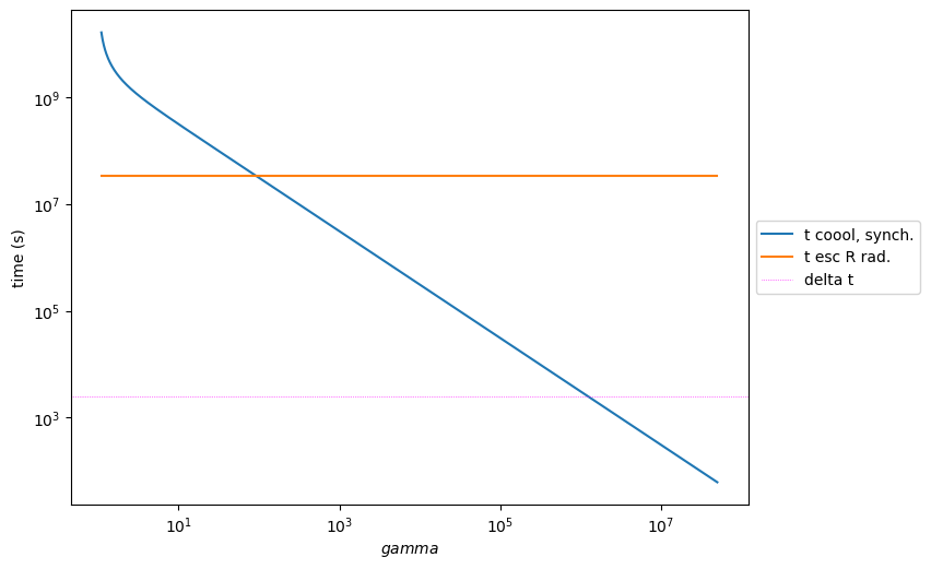
p=temp_ev.plot_time_profile()

temp_ev.run(only_injection=True,cache_SEDs_acc=False,do_injection=True,cache_SEDs_rad=False)

temporal evolution running

0%|          | 0/2000000 [00:00<?, ?it/s]

temporal evolution completed

we use the acc region with escape time equal to radiative region

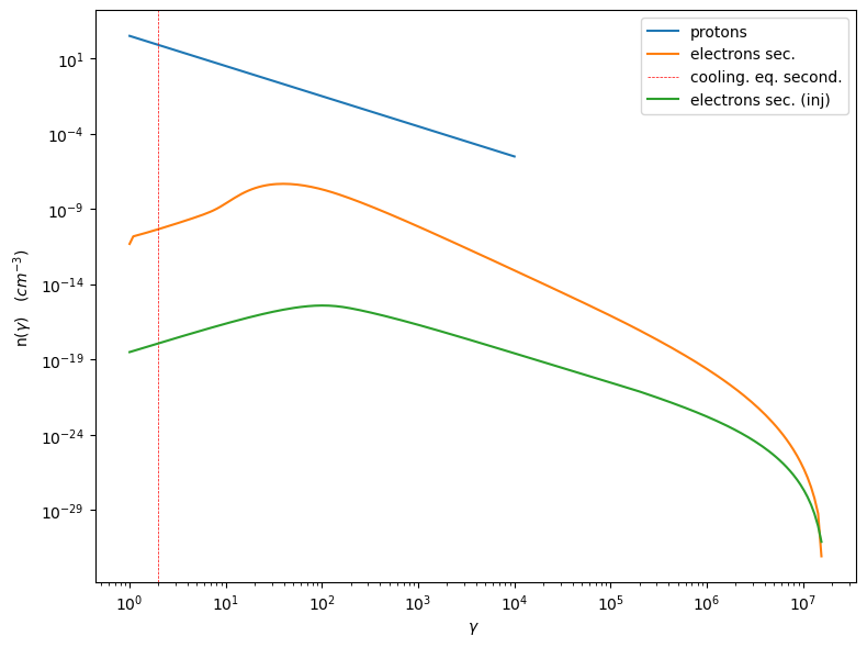
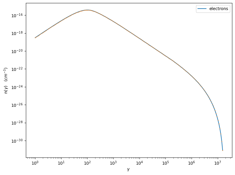
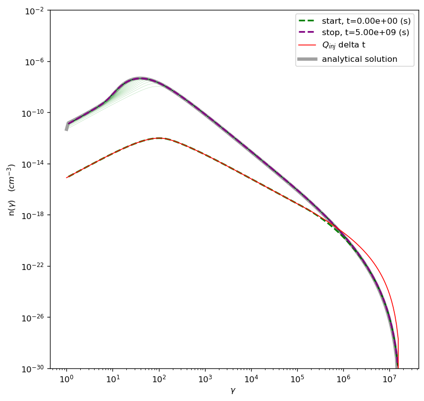
p=temp_ev.plot_tempev_emitters(region='rad',loglog=False,energy_unit='gamma',pow=0,plot_Q_inj=True)
p.ax.plot(gamma_sec_evovled,n_gamma_sec_evovled,'-',label='analytical solution',lw=4,color='gray',alpha=0.75,zorder=0)
p.ax.legend()
p.setlim(y_min=1E-30,y_max=1E-2)

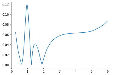
m=n_gamma_sec_evovled>0
x_analytical=np.log10(gamma_sec_evovled[m])
y_analytical=np.log10(n_gamma_sec_evovled[m])

m=temp_ev.rad_region.time_sampled_emitters.n_gamma[-1]>0
x_num=np.log10(temp_ev.rad_region.time_sampled_emitters.gamma[m])
y_num=np.log10(temp_ev.rad_region.time_sampled_emitters.n_gamma[-1][m])

y_analytical_interp = np.interp(x_num, x_analytical,y_analytical, left=np.nan, right=np.nan)

m=~np.isnan(y_analytical_interp)
m=np.logical_and(m,x_num>0.25)
m=np.logical_and(m,x_num<6)

y_analytical_interp=10**y_analytical_interp[m]
x_out=x_num[m]
y_num=10**y_num[m]

d=np.fabs(y_analytical_interp-y_num)/y_num
assert(all(d<0.25))

plt.plot(x_out,d)

[<matplotlib.lines.Line2D at 0x7fc5c4724130>]