Data format and SED data¶

The data are treated using two classes from the module data_loader

jetset.data_loader.Data class
jetset.data_loader.ObsData class

The class jetset.data_loader.Data is in charge of storing the data, giving access to the I/O functionalities, and provides an interface to the astropy Table class (see the astropy table. documentation, for further information)

The class jetset.data_loader.ObsData uses the information stored in jetset.data_loader.Data, and can perform several operations This is the class to use for model fitting and in general in Jetset

rebinning (grouping) of the data

selection of time ranges

selection of datasets

transformation from linear to logarithmic representation

handling of errors and systematics

Note

old version of data file in non ecsv astropy table format, can be easily converted by importing them using the method described in Importing from an arbitrary ascii file or numpy array to Data object and saving them

import jetset
print('tested on jetset',jetset.__version__)

tested on jetset 1.2.2

import warnings
warnings.filterwarnings('ignore')

import matplotlib
import numpy as np
import matplotlib.pyplot as plt
%matplotlib inline

Data format for Data object¶

The SED data are internally stored as astropy tables, but it is very easy to import from

ascii files
numpy array in general

once that is clear the data format. The easiest way to understand the data format is to build an empty table to have a look at the structure of the table:

from jetset.data_loader import Data
data=Data(n_rows=10)

we can easily access the astropy table

data.table

Table length=10

x	dx	y	dy	T_start	T_stop	UL	data_set
Hz	Hz	erg / (cm2 s)	erg / (cm2 s)	MJD	MJD
float64	float64	float64	float64	float64	float64	bool	bytes16
0.0	0.0	0.0	0.0	0.0	0.0	False	0.0
0.0	0.0	0.0	0.0	0.0	0.0	False	0.0
0.0	0.0	0.0	0.0	0.0	0.0	False	0.0
0.0	0.0	0.0	0.0	0.0	0.0	False	0.0
0.0	0.0	0.0	0.0	0.0	0.0	False	0.0
0.0	0.0	0.0	0.0	0.0	0.0	False	0.0
0.0	0.0	0.0	0.0	0.0	0.0	False	0.0
0.0	0.0	0.0	0.0	0.0	0.0	False	0.0
0.0	0.0	0.0	0.0	0.0	0.0	False	0.0
0.0	0.0	0.0	0.0	0.0	0.0	False	0.0

x column is reserved to frequencies (mandatory)
y columm is reserved to fluxes (mandatory)
dx columm is reserved to the error on the frequency,or bin width
dy columm is reserved to the error on the fluxes
UL columm is reserved to the flag for Upper Limit
T_start and T_stop are used to identify the time range to select data using the class ObsData
data_set

data.table['x']

0.0
0.0
0.0
0.0
0.0
0.0
0.0
0.0
0.0
0.0

columns with units are implemented using the Units module of astropy (https://docs.astropy.org/en/stable/units/).

and we can easily access the metadata

data.metadata

OrderedDict([('z', 0),
             ('UL_CL', 0.95),
             ('restframe', 'obs'),
             ('data_scale', 'lin-lin'),
             ('obj_name', 'new-src')])

z: the redshift of the object
UL_CL: the CL for the UL
restframe: possible valuesobs or src, indicating if the data are observed flux, or luminosities, respectively
data_scale: possible valueslin-lin or log-log, indicating if the data are in linear or logarithmic scale, respectively
obj_name: the name of the object

Note

starting from version 1.1.0 src to obs transformation is available

Loading from astropy table¶

you can use the default SEDs distributed with the package to get familiar with data handling

from jetset.test_data_helper import  test_SEDs
test_SEDs

['/Users/orion/anaconda3/envs/jetset/lib/python3.8/site-packages/jetset/test_data/SEDs_data/SED_3C345.ecsv',
 '/Users/orion/anaconda3/envs/jetset/lib/python3.8/site-packages/jetset/test_data/SEDs_data/SED_MW_Mrk421_EBL_DEABS.ecsv',
 '/Users/orion/anaconda3/envs/jetset/lib/python3.8/site-packages/jetset/test_data/SEDs_data/SED_MW_Mrk501_EBL_ABS.ecsv',
 '/Users/orion/anaconda3/envs/jetset/lib/python3.8/site-packages/jetset/test_data/SEDs_data/SED_MW_Mrk501_EBL_DEABS.ecsv']

As you can see there are three 3 files. We use in this example the file for Mrk 421, and we use class:jetset.data_loader.Data class

from jetset.data_loader import Data

data=Data.from_file(data_table=test_SEDs[1])

data.table

Table length=110

x	dx	y	dy	T_start	T_stop	UL	data_set
Hz	Hz	erg / (cm2 s)	erg / (cm2 s)	MJD	MJD
float64	float64	float64	float64	float64	float64	bool	str13
2299540000.0	0.0	1.3409e-14	3.91e-16	0.0	0.0	False	campaing-2009
2639697000.0	0.0	1.793088e-14	3.231099e-26	0.0	0.0	False	campaing-2009
4799040000.0	0.0	2.3136e-14	2.4e-16	0.0	0.0	False	campaing-2009
4805039000.0	0.0	1.773414e-14	1.773414e-15	0.0	0.0	False	campaing-2009
4843552000.0	0.0	2.77614e-14	2.615339e-26	0.0	0.0	False	campaing-2009
7698460000.0	0.0	3.696e-14	4.62e-16	0.0	0.0	False	campaing-2009
8267346000.0	0.0	2.836267e-14	2.836267e-15	0.0	0.0	False	campaing-2009
8331867000.0	0.0	3.98963e-14	3.627671e-26	0.0	0.0	False	campaing-2009
8388659000.0	0.0	3.16345e-14	1.931495e-15	0.0	0.0	False	campaing-2009
...	...	...	...	...	...	...	...
2.417992e+25	0.0	9.754259e-11	3.560456e-11	0.0	0.0	False	campaing-2009
3.823193e+25	0.0	8.199207e-11	7.050657e-12	0.0	0.0	False	campaing-2009
6.059363e+25	0.0	5.614334e-11	5.793969e-12	0.0	0.0	False	campaing-2009
6.073707e+25	0.0	1.14705e-10	6.573696e-11	0.0	0.0	False	campaing-2009
9.603433e+25	0.0	4.662219e-11	5.097912e-12	0.0	0.0	False	campaing-2009
1.522041e+26	0.0	5.221583e-11	4.89063e-12	0.0	0.0	False	campaing-2009
2.41227e+26	0.0	3.66834e-11	4.682033e-12	0.0	0.0	False	campaing-2009
3.823193e+26	0.0	2.247871e-11	4.343216e-12	0.0	0.0	False	campaing-2009
6.059363e+26	0.0	1.972081e-11	4.407365e-12	0.0	0.0	False	campaing-2009
9.603433e+26	0.0	7.994215e-12	3.469109e-12	0.0	0.0	False	campaing-2009

data.metadata

OrderedDict([('z', 0.0308),
             ('restframe', 'obs'),
             ('data_scale', 'lin-lin'),
             ('obj_name', 'J1104+3812,Mrk421')])

this is an extract of the astropy table saved in the format ascii.ecsv

# %ECSV 0.9
# ---
# datatype:
# - {name: x, unit: Hz, datatype: float64}
# - {name: dx, unit: Hz, datatype: float64}
# - {name: y, unit: erg / (cm2 s), datatype: float64}
# - {name: dy, unit: erg / (cm2 s), datatype: float64}
# - {name: T_start, unit: MJD, datatype: float64}
# - {name: T_stop, unit: MJD, datatype: float64}
# - {name: UL, datatype: bool}
# - {name: data_set, datatype: string}
# meta: !!omap
# - {z: 0.0308}
# - {restframe: obs}
# - {data_scale: lin-lin}
# - {obj_name: 'J1104+3812,Mrk421'}
# schema: astropy-2.0
x dx y dy T_start T_stop UL data_set
2299540000.0 0.0 1.3409e-14 3.91e-16 0.0 0.0 False campaing-2009
2639697000.0 0.0 1.793088e-14 3.231099e-26 0.0 0.0 False campaing-2009
4799040000.0 0.0 2.3136e-14 2.4e-16 0.0 0.0 False campaing-2009

Saving Data object to a file¶

data.save_file('test.ecsv')

the data can be loaded from the saved table

data=Data.from_file('test.ecsv')

data.table

Table length=110

x	dx	y	dy	T_start	T_stop	UL	data_set
Hz	Hz	erg / (cm2 s)	erg / (cm2 s)	MJD	MJD
float64	float64	float64	float64	float64	float64	bool	str13
2299540000.0	0.0	1.3409e-14	3.91e-16	0.0	0.0	False	campaing-2009
2639697000.0	0.0	1.793088e-14	3.231099e-26	0.0	0.0	False	campaing-2009
4799040000.0	0.0	2.3136e-14	2.4e-16	0.0	0.0	False	campaing-2009
4805039000.0	0.0	1.773414e-14	1.773414e-15	0.0	0.0	False	campaing-2009
4843552000.0	0.0	2.77614e-14	2.615339e-26	0.0	0.0	False	campaing-2009
7698460000.0	0.0	3.696e-14	4.62e-16	0.0	0.0	False	campaing-2009
8267346000.0	0.0	2.836267e-14	2.836267e-15	0.0	0.0	False	campaing-2009
8331867000.0	0.0	3.98963e-14	3.627671e-26	0.0	0.0	False	campaing-2009
8388659000.0	0.0	3.16345e-14	1.931495e-15	0.0	0.0	False	campaing-2009
...	...	...	...	...	...	...	...
2.417992e+25	0.0	9.754259e-11	3.560456e-11	0.0	0.0	False	campaing-2009
3.823193e+25	0.0	8.199207e-11	7.050657e-12	0.0	0.0	False	campaing-2009
6.059363e+25	0.0	5.614334e-11	5.793969e-12	0.0	0.0	False	campaing-2009
6.073707e+25	0.0	1.14705e-10	6.573696e-11	0.0	0.0	False	campaing-2009
9.603433e+25	0.0	4.662219e-11	5.097912e-12	0.0	0.0	False	campaing-2009
1.522041e+26	0.0	5.221583e-11	4.89063e-12	0.0	0.0	False	campaing-2009
2.41227e+26	0.0	3.66834e-11	4.682033e-12	0.0	0.0	False	campaing-2009
3.823193e+26	0.0	2.247871e-11	4.343216e-12	0.0	0.0	False	campaing-2009
6.059363e+26	0.0	1.972081e-11	4.407365e-12	0.0	0.0	False	campaing-2009
9.603433e+26	0.0	7.994215e-12	3.469109e-12	0.0	0.0	False	campaing-2009

Importing from an arbitrary ascii file or numpy array to Data object¶

Assume that your data are stored in an ASCII file named ‘test-ascii.txt’, with - x in the first column with frequency in Hz , - y in the second column with fluxes in erg cm-2 s-1, - dy in the third column with the same units as y - the data are in log-log scale

of course the column number depends on the file that you are using, this is only an example

from jetset.data_loader import Data
import numpy as np

d=np.genfromtxt('test-ascii.txt')
data=Data(n_rows=d.shape[0])
data.set_field('x',d[:,0])
data.set_field('y',d[:,1])
data.set_field('dy',value=d[:,2])

then you can set the meatdata as follows

data.set_meta_data('z',1.02)
data.set_meta_data('restframe','obs')
data.set_meta_data('data_scale','log-log')

of course this method applies if you have a generic 2-dim numpy array.

data.table

Table length=20

x	dx	y	dy	T_start	T_stop	UL	data_set
Hz	Hz	erg / (cm2 s)	erg / (cm2 s)	MJD	MJD
float64	float64	float64	float64	float64	float64	bool	bytes16
24.161967	0.0	-12.497324	0.334376	0.0	0.0	False	0.0
25.161967	0.0	-12.512137	0.636293	0.0	0.0	False	0.0
23.161967	0.0	-12.444346	0.38048	0.0	0.0	False	0.0
23.684845	0.0	-12.257916	0.164397	0.0	0.0	False	0.0
22.684845	0.0	-12.000541	0.0	0.0	0.0	False	0.0
15.2900346113625	0.0	-13.3225755622988	0.127157926321555	0.0	0.0	False	0.0
15.1105897102992	0.0	-12.7495312032995	0.40748532657827	0.0	0.0	False	0.0
15.1105897102992	0.0	-12.8808101179388	0.410904985836407	0.0	0.0	False	0.0
14.6702458530741	0.0	-12.477274153289	0.0	0.0	0.0	False	0.0
14.5888317255942	0.0	-12.875874154363	0.0	0.0	0.0	False	0.0
10.644439	0.0	-12.515761	0.090508	0.0	0.0	False	0.0
10.477121	0.0	-12.665868	0.072712	0.0	0.0	False	0.0
10.2988530764097	0.0	-13.2322481107094	0.486627579841286	0.0	0.0	False	0.0
10.1760912590557	0.0	-13.3326058184618	0.935000421715186	0.0	0.0	False	0.0
9.93449845124357	0.0	-13.6367199590836	0.0	0.0	0.0	False	0.0
9.92427928606188	0.0	-13.5500291112572	0.0	0.0	0.0	False	0.0
9.68574173860226	0.0	-13.7561818857395	0.427742607163214	0.0	0.0	False	0.0
9.36172783601759	0.0	-14.121068671527	0.0	0.0	0.0	False	0.0
9.14612803567824	0.0	-14.5547242324656	0.682147390735292	0.0	0.0	False	0.0
7.86805636182304	0.0	-15.4827165132972	0.025977834481891	0.0	0.0	False	0.0

Importing to Data object from a generic astropy table mapping columns¶

If you want to use a TABLE with arbitrary column names, you can use an import dictionary, mapping the input name to the target. E.g. assume that you column in the input table column named freq that should target the x column, and another named freq err associated to dx you can simply pass the dictionary to the from_file method:

data=Data.from_file(data_table='your-file',import_dictionary={'freq':'x','freq err':'dx'})

Importing from the ASI ssdc sedtool to Data object¶

To import data from a data file downloaded from the asi ssdc sedtool: https://tools.ssdc.asi.it/SED/

we can use the importing tool in the jetset.data_loader.Data. We just need to have the file downloaded from the asi ssdc sedtool, and to know the redshift of the object, the scale we selected (lin-lin, or log-log). Assume that we downloaded the data for Mrk421, in observed fluxes and linear scale, and the data are saved in the file ‘MRK421_asdc.txt’, we only have to do:

from jetset.data_loader import Data
data=Data.from_asdc(asdc_sed_file='MRK421_asdc.txt',obj_name='Mrk421',restframe='obs',data_scale='lin-lin',z=0.038)

Note

starting from version 1.1.0 src to obs transformation is available

data.table

Table length=3550

x	dx	y	dy	T_start	T_stop	UL	data_set
Hz	Hz	erg / (cm2 s)	erg / (cm2 s)	MJD	MJD
float64	float64	float64	float64	float64	float64	bool	bytes16
1.395e+17	2.077e+16	1.3665e-10	7.8618e-12	50569.13745	50569.61257	False	0.0
1.883e+17	2.805e+16	1.3231e-10	5.2986e-12	50569.13745	50569.61257	False	0.0
2.542e+17	3.786e+16	1.2801e-10	4.5958e-12	50569.13745	50569.61257	False	0.0
3.432e+17	5.111e+16	1.1696e-10	4.4475e-12	50569.13745	50569.61257	False	0.0
4.633e+17	6.901e+16	1.0488e-10	2.8152e-12	50569.13745	50569.61257	False	0.0
6.255e+17	9.316e+16	8.8421e-11	2.2462e-12	50569.13745	50569.61257	False	0.0
8.444e+17	1.258e+17	7.2995e-11	2.3614e-12	50569.13745	50569.61257	False	0.0
1.14e+18	1.698e+17	5.7982e-11	2.5232e-12	50569.13745	50569.61257	False	0.0
1.539e+18	2.292e+17	4.52e-11	2.9633e-12	50569.13745	50569.61257	False	0.0
...	...	...	...	...	...	...	...
4850000000.0	0.0	2.9604e-14	2.425e-17	0.0	0.0	False	0.0
1400000000.0	0.0	5.0638e-16	2.31e-18	49078.5	49443.5	False	0.0
1400000000.0	0.0	1.68e-17	2.296e-18	49078.5	49443.5	False	0.0
1400000000.0	0.0	8.0331e-15	2.31e-18	49078.5	49443.5	False	0.0
408000000.0	0.0	4.692e-15	0.0	0.0	0.0	False	0.0
2700000000.0	0.0	2.079e-14	0.0	0.0	0.0	False	0.0
10700000000.0	0.0	8.453e-14	0.0	0.0	0.0	False	0.0
5000000000.0	0.0	3.625e-14	0.0	0.0	0.0	False	0.0
8460000000.0	0.0	5.3433e-14	3.384e-17	47941.5	47941.5	False	0.0
8400000000.0	0.0	5.3054e-14	0.0	0.0	0.0	False	0.0

Note

When importing data from the src frame, the Data constructor will not convert units, but will assume that input units are erg/s. If this is not the case an error message will be displayed

Building the SED the ObsData object¶

Once we have a data table built with the class:jetset.data_loader.Data, following one of the method described above, you can create SED data using the jetset.data_loader.ObsData class. In the example we use one of the test SEDs provided by the package:

We start to loading the SED of Mrk 421, and we pass to ObsData directly the path to the file, because this is already in the format that we need and that we have discussed above.

from jetset.data_loader import Data
from jetset.data_loader import ObsData
from jetset.test_data_helper import  test_SEDs

data_table=Data.from_file(test_SEDs[1])
sed_data=ObsData(data_table=data_table)

if you want to use a cosmology model different from the default one please read the Choosing a cosmology model section

As you can see all the meta-data have been properly sourced from the SED file header. You also get information on the length of the data, before and after elimination of duplicated entries, and upper limits

sed_data.table

Table length=110

nu_data	dnu_data	nuFnu_data	dnuFnu_data	nu_data_log	dnu_data_log	nuFnu_data_log	dnuFnu_data_log	dnuFnu_fake	dnuFnu_fake_log	UL	zero_error	T_start	T_stop	data_set
Hz	Hz	erg / (cm2 s)	erg / (cm2 s)	Hz	Hz	erg / (cm2 s)	erg / (cm2 s)	erg / (cm2 s)				MJD	MJD
float64	float64	float64	float64	float64	float64	float64	float64	float64	float64	bool	bool	float64	float64	str13
2299540000.0	0.0	1.3409e-14	3.91e-16	9.361640968434164	0.0	-13.872603609223393	0.012663818511758627	2.6818000000000003e-15	0.2	False	False	0.0	0.0	campaing-2009
2639697000.0	0.0	1.793088e-14	3.231099e-26	9.421554078847052	0.0	-13.746398395894273	7.825876176646739e-13	3.586176e-15	0.2	False	False	0.0	0.0	campaing-2009
4799040000.0	0.0	2.3136e-14	2.4e-16	9.681154369792159	0.0	-13.635711724385564	0.0045051294803241885	4.627200000000001e-15	0.2	False	False	0.0	0.0	campaing-2009
4805039000.0	0.0	1.773414e-14	1.773414e-15	9.68169691696108	0.0	-13.751189867373059	0.04342944819032518	3.546828e-15	0.2	False	False	0.0	0.0	campaing-2009
4843552000.0	0.0	2.77614e-14	2.615339e-26	9.68516396664987	0.0	-13.556558636309997	4.091390549490907e-13	5.55228e-15	0.2	False	False	0.0	0.0	campaing-2009
7698460000.0	0.0	3.696e-14	4.62e-16	9.886403857589054	0.0	-13.43226803745193	0.005428681023790648	7.392e-15	0.2	False	False	0.0	0.0	campaing-2009
8267346000.0	0.0	2.836267e-14	2.836267e-15	9.917366113839973	0.0	-13.547252888027566	0.043429448190325175	5.672534000000001e-15	0.2	False	False	0.0	0.0	campaing-2009
8331867000.0	0.0	3.98963e-14	3.627671e-26	9.920742328771254	0.0	-13.399067379102538	3.948931348171262e-13	7.97926e-15	0.2	False	False	0.0	0.0	campaing-2009
8388659000.0	0.0	3.16345e-14	1.931495e-15	9.92369254063231	0.0	-13.499839025404517	0.026516544289422034	6.3268999999999995e-15	0.2	False	False	0.0	0.0	campaing-2009
...	...	...	...	...	...	...	...	...	...	...	...	...	...	...
2.417992e+25	0.0	9.754259e-11	3.560456e-11	25.38345485965064	0.0	-10.010805716985434	0.15852422965797036	1.9508518000000003e-11	0.2	False	False	0.0	0.0	campaing-2009
3.823193e+25	0.0	8.199207e-11	7.050657e-12	25.582426222350527	0.0	-10.086228149101405	0.03734582416192853	1.6398414000000002e-11	0.2	False	False	0.0	0.0	campaing-2009
6.059363e+25	0.0	5.614334e-11	5.793969e-12	25.78242697068017	0.0	-10.250701754501332	0.044819007294872405	1.1228668000000001e-11	0.2	False	False	0.0	0.0	campaing-2009
6.073707e+25	0.0	1.14705e-10	6.573696e-11	25.78345383740898	0.0	-9.94041765075539	0.24889236724724106	2.2941000000000003e-11	0.2	False	False	0.0	0.0	campaing-2009
9.603433e+25	0.0	4.662219e-11	5.097912e-12	25.982426510793527	0.0	-10.33140733007377	0.04748801055523926	9.324438000000001e-12	0.2	False	False	0.0	0.0	campaing-2009
1.522041e+26	0.0	5.221583e-11	4.89063e-12	26.1824263514056	0.0	-10.282197814249994	0.04067681433064456	1.0443166e-11	0.2	False	False	0.0	0.0	campaing-2009
2.41227e+26	0.0	3.66834e-11	4.682033e-12	26.38242591580127	0.0	-10.43553041856344	0.05543055158433863	7.33668e-12	0.2	False	False	0.0	0.0	campaing-2009
3.823193e+26	0.0	2.247871e-11	4.343216e-12	26.582426222350527	0.0	-10.648228615520983	0.08391205467368516	4.495742000000001e-12	0.2	False	False	0.0	0.0	campaing-2009
6.059363e+26	0.0	1.972081e-11	4.407365e-12	26.78242697068017	0.0	-10.705075251093293	0.09705961870904517	3.944162e-12	0.2	False	False	0.0	0.0	campaing-2009
9.603433e+26	0.0	7.994215e-12	3.469109e-12	26.982426510793527	0.0	-11.097224175808465	0.18846314438889974	1.598843e-12	0.2	False	False	0.0	0.0	campaing-2009

sed_data.metadata

{'z': 0.0308,
 'obj_name': 'J1104+3812,Mrk421',
 'restframe': 'obs',
 'data_scale': 'lin-lin',
 'UL_CL': 0.95}

Plotting ObsData¶

We can now plot our SED using the BlazarSEDFit.plot_sedfit.Plot class

from jetset.plot_sedfit import PlotSED
myPlot=PlotSED(sed_data)

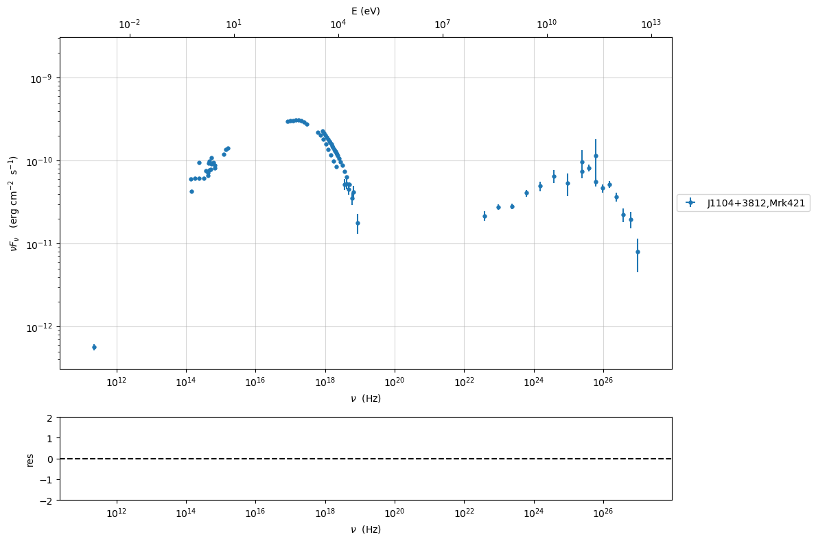
../../../_images/Jet_example_load_data_60_0.png

or you can create the object to plot on the fly in this way

myPlot=sed_data.plot_sed()

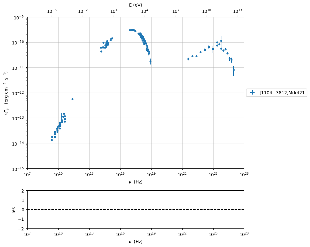
../../../_images/Jet_example_load_data_62_0.png

you can rescale your plot

myPlot=sed_data.plot_sed()
myPlot.setlim(x_min=1E7,x_max=1E28,y_min=1E-15,y_max=1E-9)

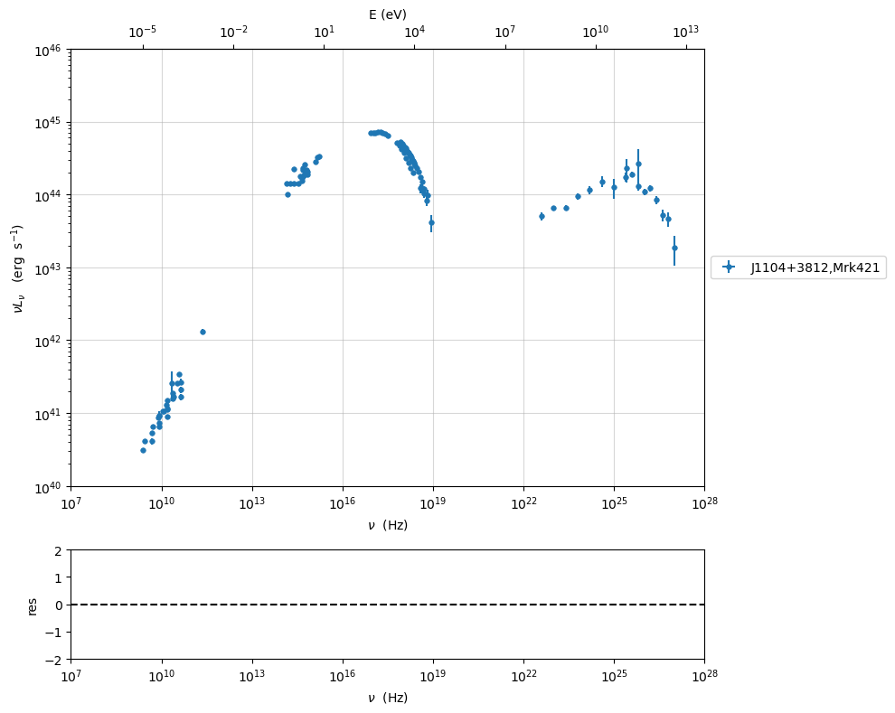
../../../_images/Jet_example_load_data_64_0.png

plotting in the src restframe

myPlot=sed_data.plot_sed(frame='src')
myPlot.setlim(x_min=1E7,x_max=1E28,y_min=1E40,y_max=1E46)

../../../_images/Jet_example_load_data_66_0.png

to have interactive plot in jupyter

if you want to to have interacitve plot in a jupyter notebook use:

%matplotlib notebook

to have interactive plot in jupyter lab use:

%matplotlib widget

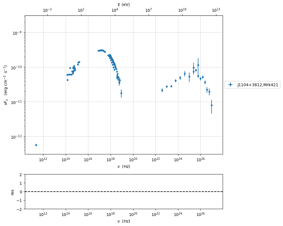
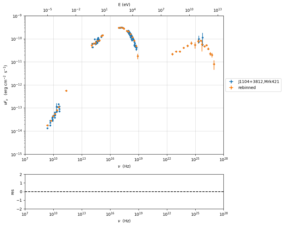
Grouping data¶

As you can see, due to the overlapping of different instruments and to different time snapshots, some points have multiple values. Although this is not a problem for the fit process, you might want to rebin (group) your data. This can be obtained with the following command:

%matplotlib inline

myPlot=sed_data.plot_sed()
sed_data.group_data(bin_width=0.2)
myPlot.add_data_plot(sed_data,label='rebinned')
myPlot.setlim(x_min=1E7,x_max=1E28,y_min=1E-15,y_max=1E-9)

================================================================================

*  binning data  *
---> N bins= 89
---> bin_widht= 0.2
================================================================================

../../../_images/Jet_example_load_data_70_1.png

Handling errors and systematics¶

Another important issue when dealing with fitting of data, is the proper handling of errors. Typically one might need to add systematics for different reasons:

data are not really simultaneous, and you want to add systematics to take this into account
data (typically IR up to UV), might have very small errors compared to those at higher energies. This might bias the minimizer to accommodate the parameters in order to fit ‘better’ the low frequencies branch.

For these reasons the package offer the possibility to add systematics

sed_data.add_systematics(0.2,[10.**6,10.**29])
myPlot=sed_data.plot_sed()
myPlot.setlim(x_min=1E7,x_max=1E28,y_min=1E-15,y_max=1E-9)

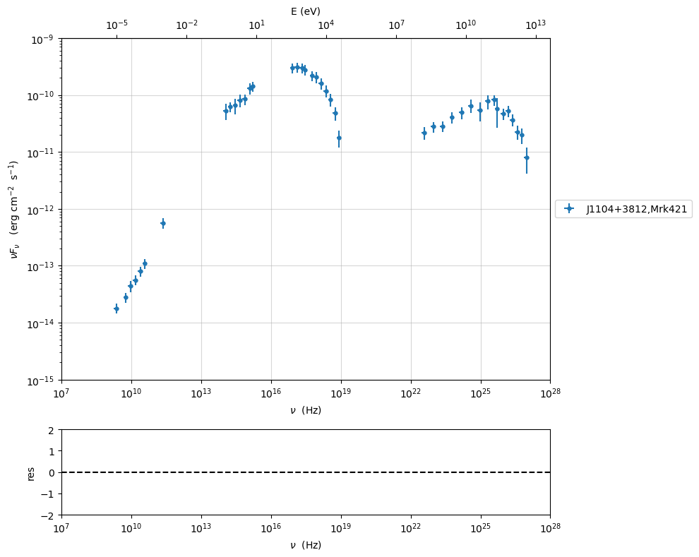
../../../_images/Jet_example_load_data_72_0.png

with this command we add 20% systematics for data between \(10^{6}<\nu<10^{29}\) Hz

Filtering data sets¶

we use the show_data_sets() method to have know wich data sets are defined in our table

sed_data.show_data_sets()

current datasets
dataset 0.0

we use show_dataset=True to have the legend of all the datasets

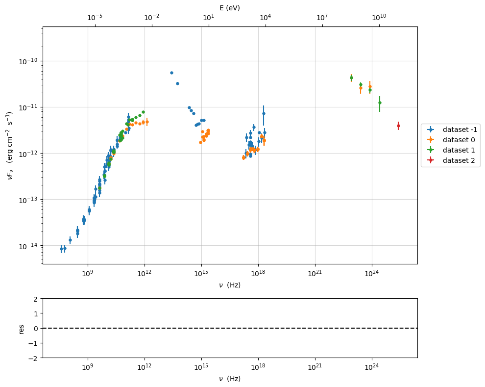
data=Data.from_file(test_SEDs[0])
sed_data=ObsData(data_table=data)
%matplotlib inline
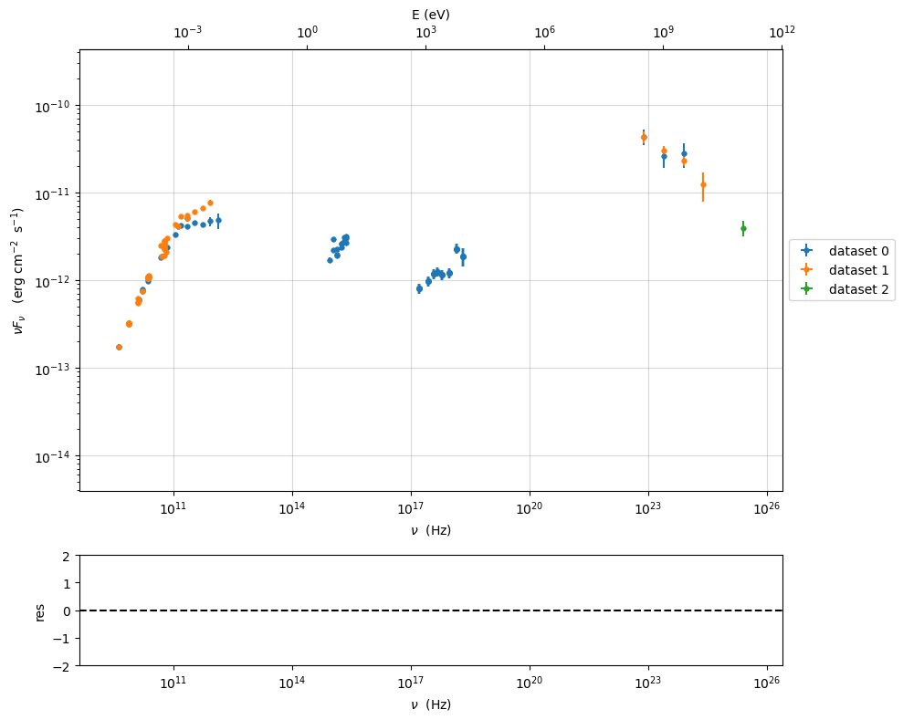
p=sed_data.plot_sed(show_dataset=True)

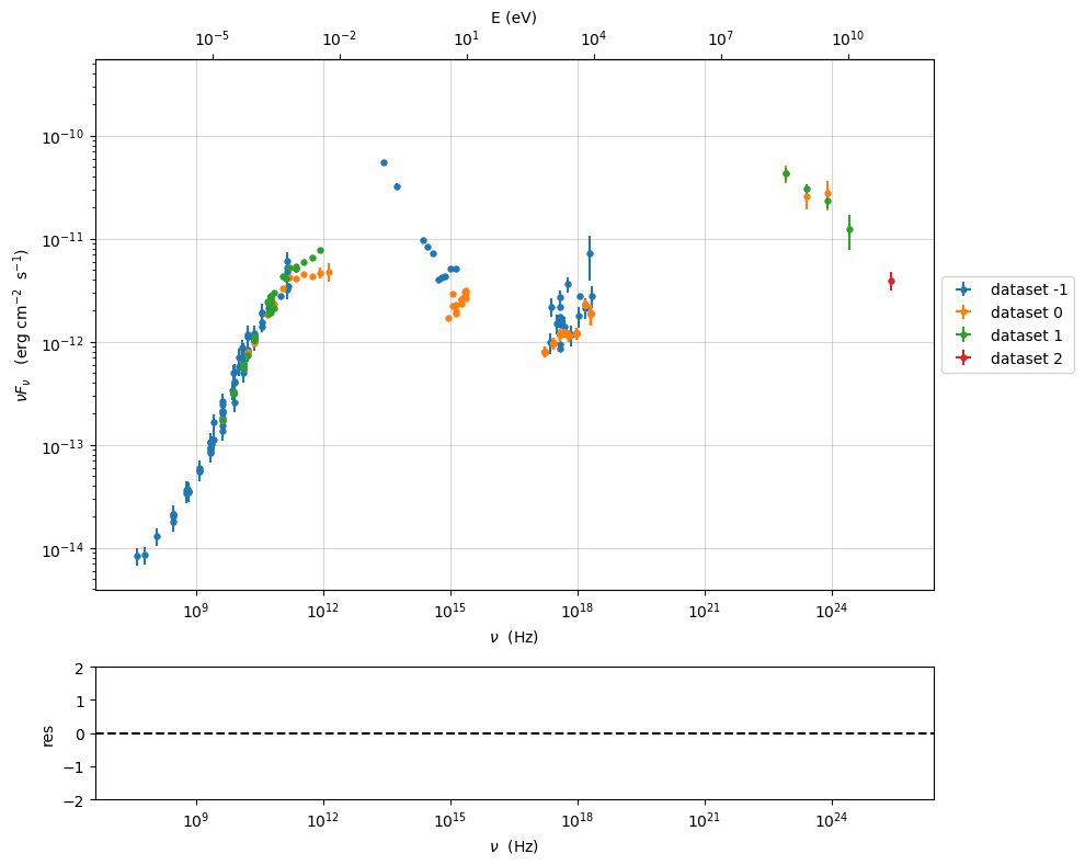
../../../_images/Jet_example_load_data_78_0.png

sed_data.show_data_sets()

current datasets
dataset -1
dataset 0
dataset 1
dataset 2

we filter out the data set -1 using the filter_data_set() method. Please not with exclude=True we exclude dataset in filters

sed_data.filter_data_set(filters='-1',exclude=True)
sed_data.show_data_sets()
p=sed_data.plot_sed(show_dataset=True)

---> excluding  data_set/s ['-1']
filter -1 192
current datasets
dataset 0
dataset 1
dataset 2
---> data sets left after filtering None
---> data len after filtering=192
current datasets
dataset 0
dataset 1
dataset 2

../../../_images/Jet_example_load_data_81_1.png

we can pass more datasets, comma separated

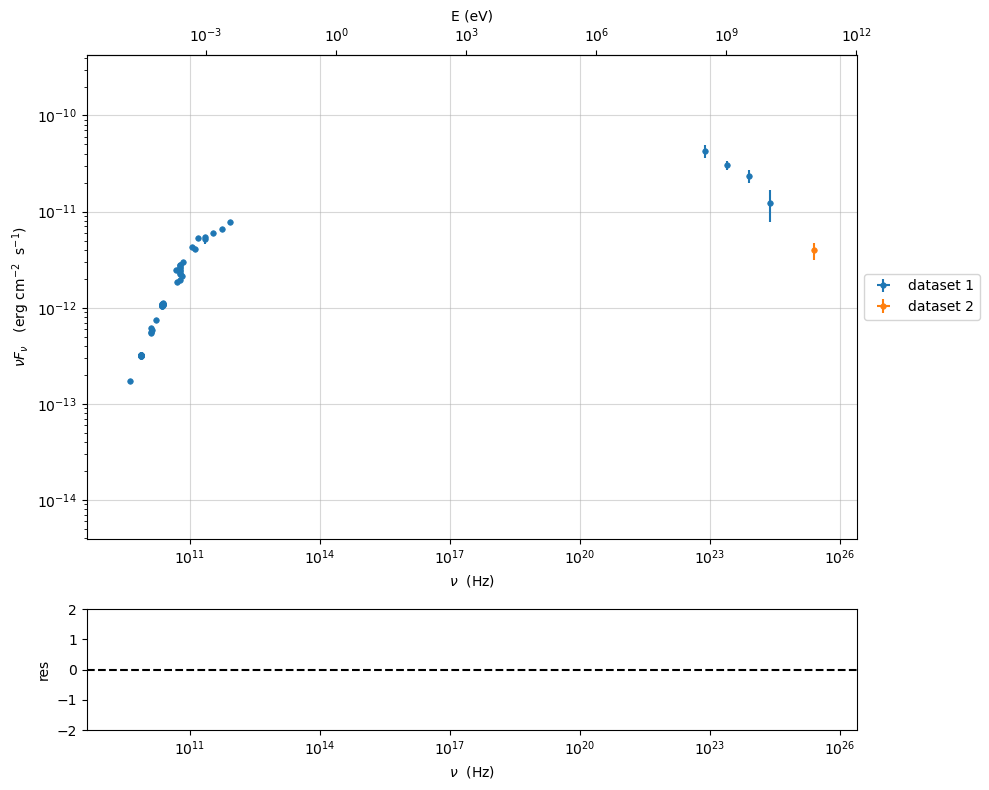
sed_data.filter_data_set(filters='-1,0',exclude=True)
sed_data.show_data_sets()
p=sed_data.plot_sed(show_dataset=True)

---> excluding  data_set/s ['-1', '0']
filter -1 192
filter 0 57
current datasets
dataset 1
dataset 2
---> data sets left after filtering None
---> data len after filtering=57
current datasets
dataset 1
dataset 2

../../../_images/Jet_example_load_data_83_1.png

we can also use filter_data_set to exclude only the datasets in filters with exclude=False

sed_data.filter_data_set(filters='-1',exclude=True)
sed_data.show_data_sets()
p=sed_data.plot_sed(show_dataset=True)

---> excluding  data_set/s ['-1']
filter -1 192
current datasets
dataset 0
dataset 1
dataset 2
---> data sets left after filtering None
---> data len after filtering=192
current datasets
dataset 0
dataset 1
dataset 2

../../../_images/Jet_example_load_data_85_1.png

we can revert sed_data to the original state with the reset_data() method

sed_data.reset_data()

sed_data.show_data_sets()
p=sed_data.plot_sed(show_dataset=True)

current datasets
dataset -1
dataset 0
dataset 1
dataset 2

../../../_images/Jet_example_load_data_88_1.png

Saving sed_data and loading¶

you can save and relaod you sed_data

sed_data.save('3C454_data.pkl')

sed_data=ObsData.load('3C454_data.pkl')

p=sed_data.plot_sed(show_dataset=True)